Distortion Tutorial

This page describes how to use the Nyquist shape function to achieve distortion.

Terminology

First, some terminology:

Clipping means that you limit the amplitude of samples, e.g.
sample_out = min(sample_in, 1.0),

or, observing that you might want to limit negative excursions as well as positive ones:

sample_out = max(min(sample_in, 1.0), -1.0).

This type of clipping is called hard clipping because the transition from an undistorted one to a maximum or minimum value is instantaneous, as if the signal hit a brick wall and can go no more.

As you might guess, you can also have soft clipping where the transition is more gradual, and that's what this tutorial is about.

Before discussing soft clipping, let's introduce a few other terms. Since clipping seems to be a way of limiting the values of the signal or compressing the range of the signal, you might think that clipping is a form of compressing or limiting; however, these terms have special meanings in the audio processing world.

Compression, or dynamics compression (not to be confused with data compression) is a way of reducing the overall range of soft to loud.

To do dynamics compression, you generally detect the intensity or peak level of a sound over a time scale of a few milliseconds, and then construct a relatively smooth amplitude control that you apply to the signal. For compression, the amplification goes down as the intensity of the input goes up, so loud passages get (relatively) softer and soft passages get (relatively) louder. (Dynamics expansion does just the opposite.) Limiters work like compressors, but are designed to eliminate peaks -- conceptually, there is no real difference, and products are often sold as "compressor/limiters". See nyquist/lib/compress.lsp for an implementation.

In some ways, soft clipping is like dynamics compression. Both reduce the gain at high levels, but dynamics compression operates relatively slowly, effectively turning the volume knob up and down, whereas clipping operates on a sample-by-sample basis. The effect of clipping is to distort the input.

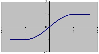
In Nyquist, you use the shape function to implement clipping. shape applies a function to each sample, where the function is specified by a sound. The following is a typical function for soft clipping:

Notice how the function is essentially y=x at small amplitudes, so there is no distortion for small signals, but at large input values, the function becomes very non-linear. Also, notice that this is similar to the behavior of real-life amplifiers, where small signals are undistorted, but at some point, the power limits of the amplifier clip the output signal.

The Nyquist shape function is allows you to specify any function you like using a sound. Therefore you can use any of the Nyquist primitives to construct the function. Since a sound is a function of time, where time must be non-negative, how do you specify a shape function over a range that includes negative values? The trick is that shape takes an offset parameter that shifts the whole function to the left (in the -y direction). Note also that whereas a Nyquist sound is generally regarded as a function of time, shape treats the sound as just a real-valued function.

The typical way to use shape is to create some increasing signal over the interval [0,2] that crosses zero at 1.0. Then you give 1.0 as the offset (3rd parameter). The result will look something like the graph above.

Implementation

In the figure above, I used a sine function to generate the smooth curve. Here is an implementation of distortion in Nyquist using the sine curve:

(setf distortion 
      (osc (hz-to-step 0.25) 2.01 *SINE-TABLE* -90.0))
(defun distort (snd)
    (shape snd distortion 1.0)) 

(play (distort (mult 15.0 (ramp 4) (osc c4 4))))

Even though I am an expert, and I have done this before, it still took me a few tries to get right. Here's a step-by-step explanation:

I used osc to generate a sinusoid so I could control the initial phase.
I set the osc duration to 2 because I want the table to go from 0 to 2 (after which we'll shift it back to [-1, +1]), but 2 is not enough because the interval [0,2] is closed, which means I need one extra sample. I used 2.01 to be conservative.
I specified *SINE-TABLE*, the default value, because the table parameter comes before the phase parameter.
I specified the phase to get the sine curve to go through zero in the middle of the generated function.
I assigned this to the variable distortion so I could plot it; try:
```
(s-plot (force-srate 100 distortion))
```
Finally, I put in a tone that ramps up from zero to 15 in amplitude to cause some serious clipping. The output amplitude is limited to 1.

Note that the input to shape is pre-clipped to the range [-1, +1] so you only need to specify the table from [0, 2] if the origin (third parameter to shape) is 1.0. If you specify a little extra, as in this example, it will be ignored.

The Output

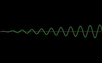
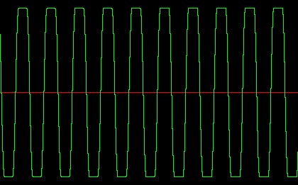
Look at the generated waveform to observe the soft clipping effect. Here we see the beginning of the output, where the input amplitude is low and there is very little distortion:

But when the input amplitude becomes large, the clipping becomes substantial. This plot is at the same scale, but taken from a later portion of the generated output. Remember that the input at this point is a high-amplitude sinusoid:

Also notice that the distortion is symetrical, so it generates even harmonics. If you put in an asymetric function, you'll get odd harmonics too. Note that at soft levels, I actually get some gain from this function.

Generated by Roger Dannenberg ([email protected]) Feb, 2004.